Data Samples

 

Adkodas data analysis: Rule extraction examples from the public domain

What sets Adkodas' AI apart from other AI is our ability to find and describe independently verifiable rules in data; here, we demonstrate on a practical level just what that means -- and what it can mean for you!

Adkodas offers customizable data analysis services: to illustrate the range of our services, below we display the results of analysis for several public data sets hosted by the UC Irvine Machine Learning Repository. These results should illustrate not only the essentials of our services but also what sort of additional investigation we can mount on your behalf; in return, Adkodas would appreciate an acknowledgment on your paper, presentation, or thesis, or even a recommendation or illustration we can post on our site.

Our first goal is to indicate the most important variables: after all, you are the expert on YOUR data, we just start by figuring out what is most important to the patterns hidden in your data and then let you independently verify why. In many cases, we can also do more than offer you the important variables; see below cases where we have found important variables and demonstrated why they were the important variables. Additionally, through the use of rule extraction we can help to identify outliers beyond mere statistical anomalies and further investigate whether they in particular are inherently different members of the data set or the result of measurement error.

Note that for best results, it is helpful for you to describe your data fields so we can verify that the analysis is reasonable; however, descriptions are not strictly necessary, if you want to run any analysis checks yourself and you are happy with results referring to your records generically (e.g. from left to right as f₀...f_n). For example, when data such as age is presented in a granular fashion, we consider whether and how to group such data into cohorts. By default, we tend to group data into a manageable number of equally-populated cohorts, but such a decision can certainly be aided by a client, if there is reason to believe a certain grouping of ages might be most relevant.

More importantly, we want you to be able to verify not only if our results match your testing data (similar to many standard neural-network analyses), but if and when the rules we extract fit with, or help to extend, the theory and understanding of your field. This is a key feature of Adkodas AI technology. While neural networks can classify data, in and of themselves they generally provide little or no information as to what outside of querying the "black box" that results; by contrast, rule extraction shows what quantities actually matter for solutions sought. Perhaps even more fundamentally, rule extraction shows in a more fundamental way not only that our neural networks work, but how they work, under what conditions they work, and without having simply try to verify that a closed black-box solution can simply replicate answers that you expect.

All data sets are different; while this may sound painfully obvious, part of the point of these examples is to illustrate not only the challenges of analyzing different data sets -- despite what is potentially or likely missing from each set -- but also that the goals of analysis may change markedly depending on the use of each set. Data and its analysis don't exist in a vacuum; there is always a specific purpose, which is why Adkodas looks to work interactively with you to help you get the most from your data, given your goals.

But on to our publicly worked examples!

 

Mushrooms

At first glance a resolution to the UCI mushroom data set may seem simple: the odor of the mushroom is the most important factor in determining whether it is edible (in particular, whether a mushroom has a smell, but not one of almonds or anise).

This may be a fine solution for avoiding poisonous mushrooms at any cost; however, when seeking a more efficient mushroom strategy, it may be preferable not to simply throw away quite so many edible mushrooms (a consequence of simply removing all mushrooms without smell).

The proportion of no-smell mushrooms that are edible to those that are poisonous is 3408 to 120; in a dataset of 8124, that could easily be dismissed as noise (or even a systematic artifact, such as the person/people collating the dataset as having a bad head cold that day). Mushrooms without smell might well be considered edible by most conventional neural networks because the error would be deemed to be "noisy" data.

But we are talking about poisonous mushrooms: people might die or become very sick if they simply eat on the basis of statistical guesswork.

This is another strength of Adkodas's tailorable data analysis solutions: being able to make a choice between generically high-percentage predictions or an analysis in which it is mission-critical to avoid false negatives or false positives in particular.

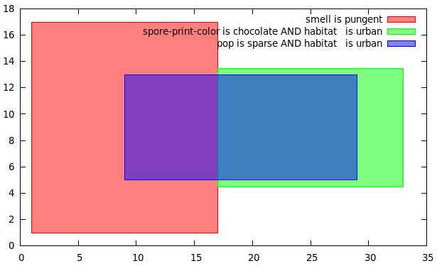
A full neural network analysis reveals that there are in fact many ways to classify the data and many rules required to do so. Some of these rules mask out other rules, as in the figure above (which shows several classes of wholly poisonous mushrooms); this is an artifact of the process rather than something we specifically try to find. Rules may overlap or intersect, and some data points contain more than one rule. Additionally, some rules are easier for humans to deal with than others; for instance, smell is often distinctively easy for humans to remember.

Our rules minimize the number of terms and maximize the number of data points they cover. To obtain all the rules, full neural network analysis is more appropriate: there is no minimization of rules (as minimization necessarily removes some information).

So how can we produce a useful and reliable simplified rule extraction, without resorting to a full neural network? First of all, we must decide on whether to concentrate on most accurately identifying edible or poisonous mushrooms. In principle the two classifications are inverses of each other, but the decision is--as we have been discussing--which identification is more mission-critical.

For example, consider poisonous mushrooms. A typical free analysis would again focus upon reporting those conditions which are most predictively correlated with the desired output (in this case, poisonous); here, those conditions are habitat and ring-type.

Additionally, input fields that seem to provide no useful information to the classification of poisonous mushrooms are attributes 1-4, 6-9, 11-14, 16-18; indeed, odor, stalk-color-below-ring, stalk-surface-below-ring, ring-type, spore-print-color, population and habitat are all the fields needed to find poisonous mushrooms. Some sample rules from these fields include the following (note that this is not a comprehensive list of found rules, nor do these sample rules cover the full data set alone, but they are provided by way of illustration):

          odor = pungent
          habitat = grasses AND (spore-print-color = chocolate OR population = several)
          habitat =leaves AND (stalk-color-below-ring = pink or white)
          ring-type is large

Here, note that odor is independent of habitat, but population and spore-print-color each depend on habitat when it comes to mushrooms being poisonous.

Additionally, sometimes it is easier to ask what something is not. Perhaps what is not poisonous is not necessarily edible. Conversely, when seeking an edible mushroom, the most important attributes are gill-color and ring-type.

The fuller list of attributes or fields needed for classifying mushroom data as being edible is attributes 5, 10, 11, 13, 15, 19, 20, 21, and 22 (odor, stalk-shape, stalk-root, stalk-color-above-ring,stalk-surface-below-ring, ring-type, spore-print-color, population and habitat), whilst the attributes that appear to be irrelevant to the classification of edible mushrooms are 1-4, 6-9, 12, 16-18.

Some sample rules for the identification of specifically edible mushrooms:

          spore-print-color is purple, orange,yellow or buff.
          ring-type is flaring

Note that the tradeoff in reported rules is a matter of elegance (capturing the most useful information in the minimal number of easy-to-apply rules) and completeness (either explaining the greatest number of positive examples, or excluding the greatest number of negative examples, depending on prioritization).

German Credit

The criteria of the German Credit data set specify a preference for declining credit to customers in the case of uncertainty of repayment: primarily a focus, then, upon negative rules. At the same time, some positive rules are clearly desirable as, in the end, "don't lend money to anyone" is not a particularly viable loan strategy.

A major challenge of the dataset is that it contains hundreds of classes of customers and not necessarily many examples of each class; amongst these are a total of 700 good credit risks and 300 bad ones.

Given the emphasis of avoiding bad credit risk, we first present an investgation on that side.

Our neural networks uncover that the most important fields for determining bad credit risk -- those that would be reported as part of a free analysis -- are those indicating whether the applicant has a phone registered in his or her name and what his or her job is. (Notably, this means that the data set is showing its age, given that "having a phone" would be, to say the least, unlikely to be a primary consideration today.)

A more detailed neural network analysis reveals a significant number of more detailed rules, including some examples given here:

     age <= 25, other installment plans at the bank and you are an unskilled citizen
     age <= 25, you are an unskilled citizen and a phone registered in your name
     there is a co-applicant, you rent and you already have an existing credit at the bank

     other debtors/guarantors of a co-applicant AND renting AND the number of existing credits at this bank is 1

     age <= 25 AND job=unskilled resident AND (other installment plans at a bank OR telephone registered under the customers name)

Fields not relevant to determining whether a client is a bad credit risk include the status of existing checking account, the duration of the loan, and (interestingly, for this data set) credit history. (This is one of the primary powers of neural network analysis, at times -- to identify unintuitive predictors, both those which are presumed unhelpful, but perhaps even more crucially, those which are erroneously presumed helpful.)

Added complexities soon surface: purpose of the loan only matters for bad credit when it's for a new car. Conversely, purpose of the loan only matters for good credit risk when for furniture or equipment.

More generally considering good credit risks, the most critical fields (and again, the typical result of a free analysis) is whether a client has a registered phone line and whether a client has any other existing credits at this bank.

The status of existing checking account, duration in months and credit history are again irrelevant to the data set, which is not surprising given the symmetrical nature of the question.

A few sample rules of good credit risks are:

     you have over 1K in savings AND number of credits at the bank is 1 AND how many dependents you have is 1.


     You are a foreign worker (presumably, a legal-resident situation) AND 
     (unskilled worker resident OR number of dependents is 2)

While the data set (and conclusions from it) may be dated, the extraction illustrates the most salient points of good and bad risks within the data. Because of the large number of classes -- and likely also because of the familiar problem of other information, masked out, that would also determine whether a customer is a good credit risk -- no single compact set of rules will suffice to completely quantify the creditworthiness of a single prospective customer.

However, while there are hundreds of total rules and hundreds of classes of data in this data set, many ill-populated, our full neural networks can learn this data set perfectly in seconds and then test potential customers quickly to see if they make a good credit risk.

Forest Fires

The UCI forest fires data set is different from the others considered thus far in that identical starting conditions can produce different outcomes: specifically, the same input conditions are reported in one line of data in which there may be no fire and then again in another line of data in which there is a small or large fire.

The cause of this is, of course, usually missing information; notably, in this case, a large number of fires are the result of human activity. Other background factors (e.g. the number of grazing animals keeping down the level of potential kindling) or even more random factors (e.g. lightning strikes) also doubtlessly contribute. Obviously, factors not included in the data set are impossible to directly resolve through data analysis.

These caveats aside, the most obvious predictive factor, as found by our neural networks, is the location on the map, primarily the x coordinate and secondly the y coodinate. (This information would be included in our free service; what beyond that, as the continuing discussion unfolds, would depend on what is specifically sought to learn from this data.) These conditions make sense, insofar as they relate to the accessibility of the location (either to start or to fight the fire).

The size of the fire was divided into roughly equally-populated classes (measured in ha, or hectare = 10000m² or approximately 2.47acres), except for class 0, which had many more examples than any other class.

     If the area burned was 0 ha (hectare, and specifically less than 100 m2 were burned), then it is class 0. 
     If it burned more class 0 but less than 2 ha, class 1. 
     From 2 to 5 ha, class 2. 
     From 5 to 10 ha, class 3. 
     From 10 to 50 ha, class 4. 
     More than 50 ha, class 5. 

For comparison, the US National Wildfire Coordinating group classifications:

     < 0.25 acres is class A ( about 10x the size of the 0 size fire for this data set)
     0.25 to 10 acres is class B (0.1 to 4 ha)
     10 to 100 acres is class C (4 to 40 ha)
     100 to 300 acres is class D (40 to 120 ha)
     300 to 1000 acres is class E (120 to 400 ha)
     1000 to 5000 acres is class F (400 to 2000 ha)
     > 5000 acres is class G (2000 ha or bigger)

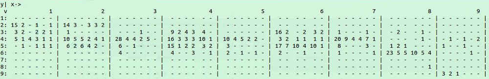
In the table below, counts represent the number of each type of fire (classes 0-5, individual columns between dividers) for each x-coordinate (divided columns) and each y-coordinate (rows).

In particular, for many of the y-coordinate locations no fires were recorded at all, namely 1 and 7, as well as very few were located in 8 and 9. While in general this may not be surprising versus a map of the park for which these fires were collated, even the low number of fires in 9 is somewhat surprising given it is even more remote than than y-coordinates 1, 7, and 8.

The other features in the data that our networks found to be important are the temperature and especially the relative humidity (with higher numbers of fires concentrated between RH of 35 and 45%).

While it would be helpful to determine a universal equation that predicts the size of a fire based on temperature, rain, RH and wind speed alone (in particular, independent of specific location and terrain), e.g. along the lines of the effort of A Data Mining Approach to Predict Forest Fires Using Meteorological Data by Cortez & Morais, it is not possible from this data set alone, due to its particularly strong geographical correlations - which implies that geography generally may be as, or even more, important a predictor as meteorological quantities.

While identifying the most important correlations is, of course, an important research tool, for direct predictions based upon a particular area -- especially here for medium-grade and larger fires -- there are also our full neural networks.

E. coli

In the UCI E. coli data set the challenge is finding an automated way to distinguish between 8 classes of e-coli. For simplicity each class of E. coli is numbered 0-7.

Our analysis found that this data set has 7 useful attributes or input data fields with which to distinguish the e-coli:

     0. mcg
     1. gvh
     2. lip
     3. chg
     4. aac
     5. alm1
     6. alm2

To be able to fully differentiate between all the E. coli all of these seven attributes were needed. For example:

To distinguish between E. coli types 6 and 7, attribute 4 (aac) is all that is required.
To distinguish between E. coli types 0 and 6, attribute 0 (mcg) is all that is required.
To distinguish between E. coli types 0 and 1, types 0 and 4, types 1 and 2, and types 2 and 4, the required attributes are 0, 1 and 4 (mcg, gvh, and aac).

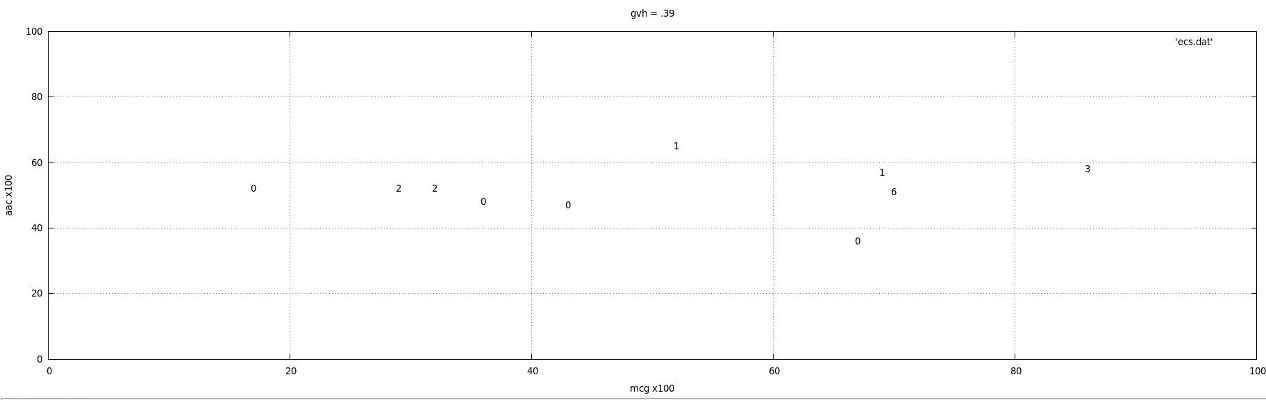
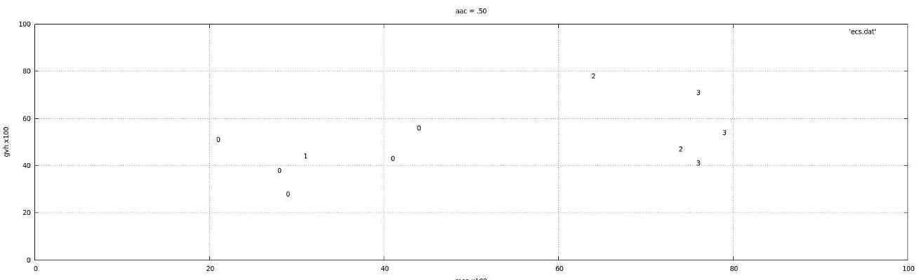
A convoluted 3D surface separates classes 0, 1, 2 and 4 of E. coli; see, for instance, the "snapshot" diagrams below for specific values of attribute 1 (gvh=0.57, gvh=0.39) and attribute 4 (aac=0.50); numbers denote different classes. Particularly in the first diagram, we see that when gvh is .57 there is strong separation between the kinds of E. coli,but the boundaries separating classes are not linear/planes.

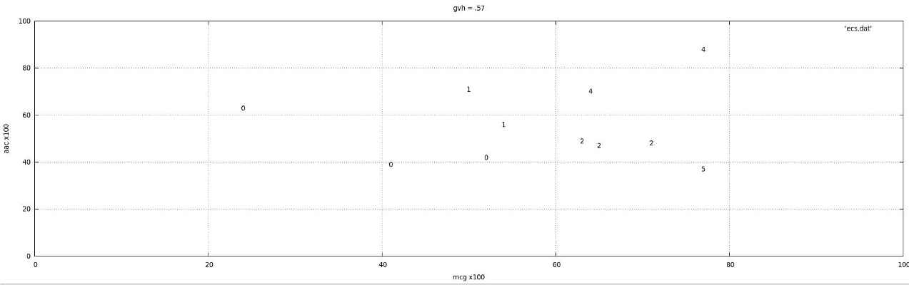
No pair of types of E. coli need all 7 attributes to distinguish between them.

Using our full neural networks we get an error rate of about .09 (when data points were randomly selected for testing from all classes of E. coli) when training with 90% of the data set (with error predominantly among types 5, 6 and 7 because they have so few data points--hence the neural network has trouble distinguishing them).

Wine analysis

The UCI wine data set includes a chemical analysis of 13 attributes of 3 different kinds of wine (each derived from its own cultivar).

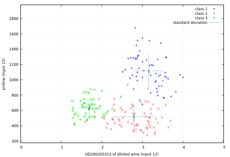
The most immediate result is that for all three output classes, the attributes that matter most are inputs 12 and 13: OD280/OD315 of diluted (x-axis) wines and proline (y-axis). While there is some overlap in the total range of each wine type, there are distinct concentrations in these two parameters that well define the differences between the three classes.

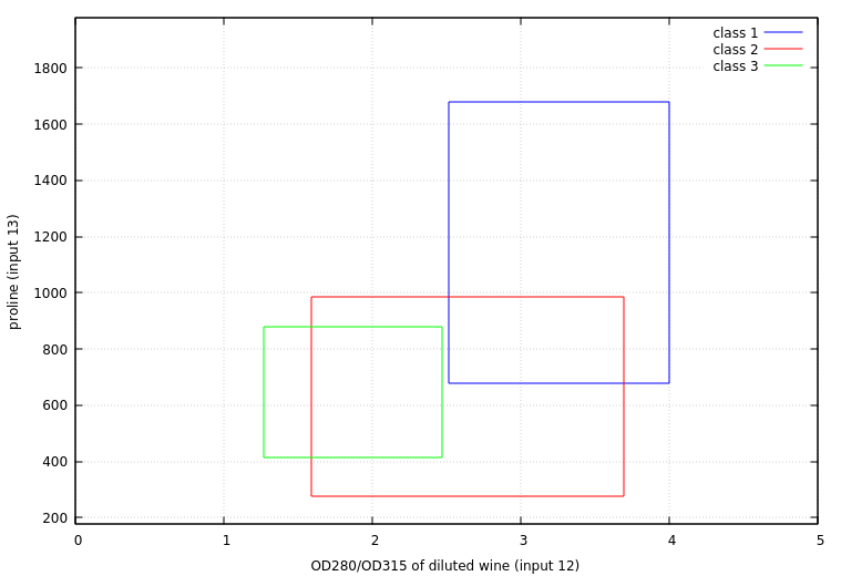
While the total range of parameters for each wine type gives a sense of the possible classification scheme, a better measure of how much overlap there is between types can be demonstrated by looking at the mean values (marked with wine type numbers) and standard deviation (marked by error-bar lines) for each parameter, showing that the true extent of overlap -- points occuring within one standard deviation of another wine type's mean value -- is relatively minimal.

In Conclusion

Adkodas' free services can be tailored with reasonable limits to fit you want, but center around the power of our neural network rule extraction to allow you to make your own visualizations (similar to those above). If you seek aid in constructing visualizations, or need access to the full power of our neural networks, contact us to negotiate a paid full-service solution!

Legal    Privacy   Contact Us